Go back to ObjectJ Examples
version 04g
01-Apr-2022
News
Download
Utilities
Explanation of results
Coli-Inspector is a project that analyses phase-contrast and fluorescence images of bacteria, and runs under ImageJ in combination with plugin ObjectJ.
It uses composite objects to combine many different parameters per cell.
Norbert Vischer
Bacterial Cell Biology
University of Amsterdam
vischer at uva nl
Automatic Measurements:
- Length and diameter of filamentous bacteria
- Fluorescent spot positions in local coordinates
- Constriction sites
- Maps of profiles
If not done yet, install ImageJ from: http://imagej.nih.gov/ij/
If the ObjectJ plugin is already visible under menu Plugins, jump to (4).
Otherwise, you can install it as follows:
Download objectj_.jar and drag it onto the ImageJ main window (that also contains the tools).
ImageJ then suggests to store it in the plugins folder.
Confirm by clicking the Save button.
You can choose Plugins> ObjectJ to make the ObjectJ menu visible (see fig 2),
but the ObjectJ menu will appear anyway the first time you open an .ojj project file.
Download and unpack the folder 'Coli-Project', which containins two hyperstacks. We will use it as our 'project folder'.
Download and unpack the project file 'Coli-Inspector-xx.ojj' and store it in the project folder mentioned above.
Download
In order to open Coli-Inspector-xx.ojj, you can either drag it from the Finder/Explorer into the ImageJ main window, or you can use ImageJ's Open menu.
If the ObjectJ menu (between Analyze and Plugins) was not visible yet, it should appear now.
Now the project window is shown, with the panel for linked images still being empty.
In order to link the two files Cells_1.tif and Cells_2.tif, go to the Finder/Explorer and drag them into "Linked Images" panel (Fig 2). Alternatively, you can link images via menu ObjectJ>Linked Images.
The two green bullets confirm that the image files are in the same folder as the project.
The hyperstacks used here contain, besides the phc channel, only one fluorescence channel, but your own files may contain multiple fluorescence channels.
Now you can start with the analysis, using the embedded macro commands under ObjectJ menu.
Choose ObjectJ> Mark Filaments (which is the first embedded macro)
It measures all 6 phase contrast images contained in the two hyperstacks, and indicates which criteria are not met in case of rejection (Fig 3)
It also calculates profiles for diameter and fluorescence along each cell. These profiles are stored in profile maps (Fig 4).
Via ObjectJ> Constrictions and Spots.. you can add more parameters per cell.
Constrictions are marked with yellow dots in phase contrast (Fig 6).
Fluorescent Spots are marked with magenta dots in in the corresponding channel (Fig 7).
Choose ObjectJ> Show ObjectJ Results to study the results (Fig 8).

Fig 1: Project file (ending with .ojj) and images need to be in same folder

Fig 2: Left: ObjectJ Tools indicates item types Axis, Dia, Const and Spots that are used for marking.
Right: 'Linked Images' panel of project window shows that two stacks (Cells_1 and Cells_2) are linked. Green bullets indicate that the files are in the correct folder.

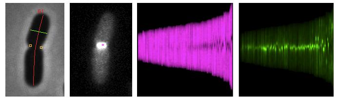
Fig 3: Automatic marking of cell axis (red) and diameter (green). Rejected cells are temporarily labeled in yellow.

Fig 4: Evaluation area for fluorescence profiles along the cells

Fig 5: Profiles of 129 cells are displayed as "Map", which is 130 pixels wide. Each cell is displayed as a vertical line.
Magenta: intensity corresponds to local diameter, constricting cells are dark in the middle. Where title indicates "Sorted", cells are sorted for cell length (age increases towards right).
Green: intensity corresponds to local fluorescence (again sorted).
Select the "M" button in ObjectJ Tools (right) and click in the map to reveal the corresponding cell.

Fig 6: Makers for axis, diameter and constrictions in phase contrast

Fig 7: Tolerances for SpotFinder: you can avoid the dialog by replacing zeroes with fixed values in variable noiseToleranceSpots[].

Fig 8: ObjectJ> Show ObjectJ Results shows linked results. Each row is connected to the cell with the same numeric label, and will disappear when you kill the cell.
Show explanation of result columns

Fig 9a: ObjectJ> Collective Profile Settings
Derives profiles from current Map. If "Age Group To Resolve" is > 1, the "Age" column is used to subdivide the population in equally spaced age groups, shown as a stack of profiles. "Age" is derived from cell length via "Update Map-Dependent Results".
If "Normalize to yMax=1" is FALSE, only one channel can be plotted, and then you also can specify Y-Range manually by using a value other than 0.

Fig 9b Top Right: Leader (chn2) is rotated so that the strong pole appears in the left half of the plot. Other channels follow.
Fig 9b Bottom: Age groups to resolve = 3: population is divided into group, resulting plots appear in a stack of 3 slices.

Fig 10: ObjectJ> Plot Collective Profiles
Stack of 5 profile plots is shown with the first age group (Age = 0..20%) in front.
Show Mirror Plot of Channel 2: Channel 2 shows its mirror image as thin green line in order to illustrate the deviation from symmetry.

Fig 11: ObjectJ> ScatterPlot: Spot Positions Dialog Scatter plot spot position vs axis is painted for all checked spots. Set Leader Channel > 0 to put strong poles to the top- other channels will follow the leader.

Fig 12: ObjectJ> ScatterPlot: Spot Positions
This project has embedded macros (macro text is editable via ObjectJ> Show Embedded Macros), which appear indented in the ObjectJ menu:
Mark Filaments
Marks cell axis and mean diameter of the cylindrical cell part. If a "Contour" item is listed in Tools, the cell contour is marked as well. Marking takes place in phase contrast channel of all linked images. Reasons for rejected cells are temporarily shown as orange text overlay.
The ObjectJ results table is automatically populated with corresponding values (e.g. Axis = 3.5 um, Dia = 0.9 um).
Additionally, a map of profiles is created and stored as 32-bit hyperstack in the project folder. In the map, each cell is represented as a single column of pixels, whose height equals the length of the cell axis. The individual pixels contain either the local diameter (in case of phase contrast), or fluorescence of a disk 1-pixel-thick (in case of fluorescent channel). Depending on "intFluorFlag" in embedded macros, fluorescence is either mean or (by default) integrated fluorescence. Cell#1 is located at x=1 in the map, cell#2 at x=2 etc.
Spots and Constrictions...
Add Single Constr's to Chn 1
one central constriction per cell is detected from channel 1 in the Map mentioned above, and marked as an invisible ObjectJ marker line with visible end points (orange). The length of the line is displayed in the ObjectJ results (e.g. Constr=0.6 um).
Add Multiple Constr's to Chn 1
several cell constrictions are detected from channel 1 in the Map mentioned above, and marked upon the cell as an invisible ObjectJ marker line with visible end points (orange). The number of constrictions per cell is displayed in column "nConstr" in the ObjectJ results.
Delete constrictions
Deletes all constriction markers
Add RSpots to channel 2
This command starts the MaximumFinder and guesses noise tolerance to detect spots in channel 2. Once a noise tolerance is chosen, spots are marked with dots of type "RSpot" in channel 2. The program automatically arranges item types that end with "Spot" to increasing channels, starting at channel 2.
Spots in the correspondig channel are marked with dot markers.
You can override noise tolerance guessing with fixed values in the embedded macros.
Delete RSpots
Deletes all RSpots
Rebuild Map
Any old Map of profiles is discarded and recreated, using the existing cell markers (axis and diameter). This may be useful if the map is lost or damaged.
Compact and Show Map
The Map of profiles is compacted (removing killed cells), and displayed.
Sorted and Qualified Map
The user is asked what to sort. Usually, we sort for Axis. Then the map shows shortest cells left, longest right. Only qualified cells are included.
Update Map-depending Results
Compacts the Map and extracts cell parameters (like cell volume) from it, which then will be written to the ObjectJ linked results table. In order to make the ObjectJ results table not too complex, only parameters of one fluorescence channel (eg channel 2) can be displayed at a time. Three different 'advance' levels can be chosen, providing an increasing number of derived result columns (press Help button for explanation). This command also creates an "Age" column, that derives age by default from cell length assuming exponential growth of a steady-state population (not qualifier dependent).
Display Mode (Composite/Gray) [D]
Toggles display mode between current channel and all channels - a shortcut for: Image>Color>Channels Tool..
Show/Hide Outlines [F6]
Recreates the rois as used by the particle analyzer as one single composite roi (including rejected rois). Run this command a second time to hide outlines (or choose Edit>Selection>Select None).
Navigate >
Zoom to Previous Object [F1]
If an object is selected, the previous object will be selected and shown in zoomed mode. Note that the terms "Next" and "Previous" respect sort modus. E.g. if sorted for "Diameter min at top", "Previous" means the "Show the next thinner cell"
Zoom to Next Object [F2]
Selects next object and shows it in zoomed mode
Zoom to Current Object [F3]
Shows selected object in zoomed mode
Zoom to Object#... [F4]
Use Virtual Stacks for Browsing [F5]
Opens all linked images as virtual stacks.
Especially useful when browsing in sorted mode, as jumping from image to image needs not to open them in a new window.
Advance [A]
During manual marking, next item type in ObjectJ Tools window is activated, and corresponding image channel for this item type is chosen (e.g. channel 2 for RSpot)
Close Object [C]
During manual marking, any open object (indicated by italic label with asterisk) is closed. This is a keyboard shortcut for the "Close" button in ObjectJ Tools window
Kill [K]
Kills currently selected object and shows next object in zoom mode. An alternative way to kill an object is using the pistol from ObjectJ Tools
Reverse Axis [R]
Reverses the direction of selected cell's axis and puts its number label to the opposite side.
Calculate Spots
Spot positions are displayed in local coordinates.
Scatter Plot: SpotPos vs Length
You can choose which types of fluorescent spot positions are plotted versus axial position.
Plot Collective Profiles
A Map needs to be in front, then the desired channels of the Map are used to create cumulative plots. All profiles are resampled by default to 101 pixels (i.e. cell length is normalized), and then averaged for each age group. If AgeGroups > 1, profiles are arranged as stack, and data can be copied or saved via a text table (Use Edit> Options> Input/Output.. to in/exclude headers or row numbers). There is a choice to mirror profiles so that the stronger pole of the leader channel is always in the left half of the plot; other channels will flip if the leader channel flips. Cells that are not represented in the front map will not be included, i.e. you can use qualifying to make profiles of subsets.
Subtract Fluor. Backgrounds ..
From all linked fluorescent channels, backgrounds are calculated (as modal value of central 80% of width and height). With key Caps Lock down, the observer will see those pixels in red which would become zero after background subtraction. Before performing any subtraction, a table of calculated backgrouds is shown, with the option to edit the table or abort the process. The table is also copied to the clipboard, and if the user chooses File>New>System Clipboard, there are more options to edit than only to delete rows. However, the table columns may not be properly aligned.