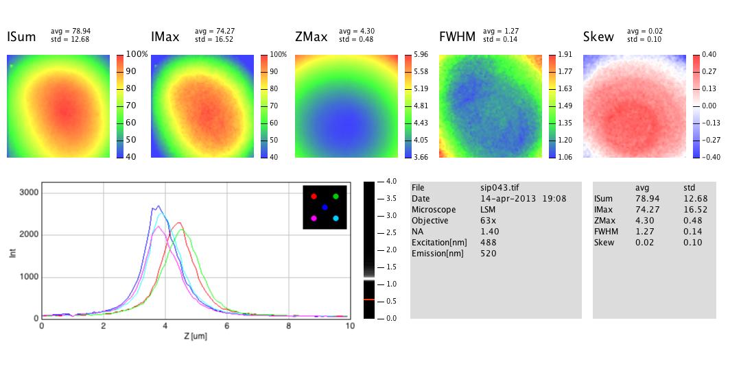
SIPchart plugin for ImageJ

Norbert Vischer

G.J. Brakenhoff
Mark Savenije
University of Amsterdam
https://sils.fnwi.uva.nl/bcb/sipcharts/SIPchart.html

date: 26-jan-2016

Fig. 1: SIPchart

Introduction

A SIPchart is suitable to quantify the sectioning quality of a confocal microscope. It is obtained by processing the 3D image of a thin fluorescent layer. This documentation describes the SIPchart plugin running under ImageJ.

Before creating the first SIPchart from a 3D image (also called "stack"), it is necessary to install the ImageJ application (on Windows, OS X, or Linux) and to download the plugin "SIPchart_.jar" .

For ImageJ look here:
http://imagej.nih.gov/ij/

Installation:

1. Make sure ImageJ is installed and open.
   
   
2. If "SIPchart" appears already under menu Plugins, skip next two points
   
   

3. Download the 'SIPchart_.jar' plugin. Make sure that it has not been renamed (some browsers append a suffix number if an older version exists in the download folder).

4. For installing, drag SIPchart_.jar onto the ImageJ main window (which contains the tools). Confirm "Save" when ImageJ asks to save it in the plugins folder.
   Under menu "Plugins", now "SIPchart" should be listed.
   
   

5. Choose menu Plugins> SIPchart
   This installs two icons "SIP" (the tool menu) and "PL" (the "Plot Live" tool) as shown below in Fig. 2. (You also can re-install the tools this way if they were removed).

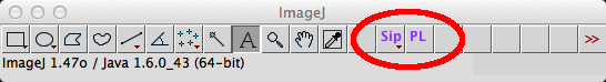
Fig. 2: ImageJ main window with tool menu "Sip" and "plot-live" tool "PL"

Run the demo:

1. Download the demo stack sip043.zip, and open it in ImageJ (ImageJ also accepts zip-compressed stacks). Note that tool menu Sip> Load Demo Stack From Web does not work anymore and will be removed in the next version.
   The demo stack contains 100 slices
   
   

2. Choose tool menu Sip>Make SIPchart
   SIPchart is built within seconds as shown in Fig.1.

3. Select the Plot Live tool ("PL") from the tool bar and click on any of the colored panels, or inside window "PanelStack":
   When clicking and dragging the mouse inside "PanelStack", a live plot will be created (Fig. 3)and show the through-Z plot for the corresponding x-y position.

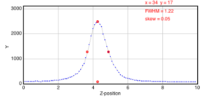
Fig. 3: Live profile while dragging mouse across PanelStack

Use your own image:

• Open your stack in ImageJ

• If your z series is not organized as stack yet - choose menu File > Import> Image Sequence in order to create a stack from individual images.

• If necessary, choose Image>Transform> to flip horizontally, vertically, or Z. - in case your microscope uses different display conventions for left/right, back/front, up/down.

• Choose menu Image>Properties and make sure that voxel size is entered correctly,

• Optionally, choose menu Plugins>Macros>Set Microscope Specs
  Here you can to enter lens and instrument data - they will appear in the output plot. If NA, Excitation and Emission wave lengths are entered, the program will draw the theoretical FWHM limit as red line into the resolution bar.

• Optionally, choose menu Plugins>Macros>Add Microscope Specs from Clip so you can re-use specifications from clipboard without re-typing. The clipboard could for example contain lines like below:
  
  Microscope=Zeiss IV
Objective=63x
NA=1.40
Excitation[nm]=488
Emission[nm]= 520

Create SIPchart:

with the stack in front, choose tool menu Sip>Make SIPchart

The SIPchart will be created within a few seconds. (Please don't disturb the process with mouse clicks inside ImageJ windows).

The program will performs the following actions:

Before creating the charts, the source stack is downscaled to x * y = 64 * 64 pixels using bilinear interpolation. The prefix "binned-" will be added to the original image name. If the original image is not square, only the largest centered square will be evaluated.

From each xy position, a z-profile will be analyzed:

Results are stored in a "PanelStack" containing five 32-bit images (you can navigate between ISum, IMax, ZMax, FWHM, Skew). Each slice holds the corresponding parameters for all x-y positions. The status bar shows the parameter that belongs to the current cursor position and panel.

The final SIPchart is composed of these five panels in false color, a resolution bar (histogram of FWHMs), five z-profile plots (at image center and four quadrant centers), plus a textual summary. Numerical output is stored as metadata in the chart, and will be preserved if you store the file in .tif format. You can make it visible via tool menu Sip> Show Numerical Results and copy-paste it to a spreadsheet, or re-use it for the microscope specs.

PL-Tool (Plot Live) and Live Profile:

The PL-tool appears in the main ImageJ window with a "PL" icon (see figure). Activate this icon and click on the "PanelStack": the status field shows the corresponding numeric value under the mouse (e.g. FWHM in mocrons if the FWHM channel is activated). Click and drag to obtain a live z-profile plot.

Technical information The algorithms used here are simple and performed in a few seconds. Results match well with the former server-based SIPchart programme. As this plugin is open-source, more sophisticated algorithms can be appended. The source code is included in the SIPchart_.jar file.

Current algorithm: Peak height and position are obtained by a polygon that represents the tip (top-most 25% of profile). Its center of gravity (cx, cy) is calculated. PeakpositionX = cx PeakMaximum = cy/0.85 The FWHM points are found where the profile crosses half maximum. The Skew is calculated from (b-a)/(b+a), where a and b are left and right width of half maximum, respectively. Backgroud is calculated from the lowest values found in first and last slice of the binned image.