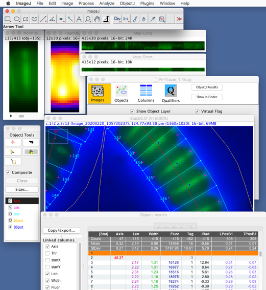
Fig 1: Overview
https://sils.fnwi.uva.nl/bcb/objectj/examples/Fil-Tracer/MD/Fil-Tracer.html
29-Sep-2021 version 1.4i
N.Vischer
Fil-Tracer is a software project that runs under ImageJ with plugin ObjectJ.
It was written to resolve and analyse multicellular bacteria like human-associated Neisseriaceae. These cells divide longitudinally and are arranged as filaments, so that a cell's long axis is perpendicular to the filament's axis. ObjectJ's special feature of embedded macros, composite objects and linked results allows to resolve, mark and analyse the cells without loosing the connection to the filament markers.
Download project file and demo images
Fig 1: Overview
Description of ObjectJ menu commands:
ROI to Island [F1]
Expects a freehand selection on the linked front image and converts it to an ObjectJ Item of type "Island" (yellow contour). An island should exclude filament crossings, kinks, and other problematic areas.
Mark Filament Axes
Removes all non-Island Items (i.e. previous axes etc). Then, applies the particle analyzer to all slices in channel 1 and marks the filament axes as "Axis" items (red lines).
Mark Cell Boxes
Resolves cells from the marked filaments and marks each with a trapezoid-like polygon of type "Box" (color = cyan).
The numbered poles are all at the same side of the filament axis, at the dominantly convex side (outside).
Mark Cell Lengths
Detects maximum gradient per box and marks the cell axis as type "Len". The line (color = magenta) follows the symmetry axis of the cell box.
Calc intensity Chn2
Measures the mean value of each box in channel 2.
Mark Spots
Finds maxima in channel 2 and places one or several "BSpot" markers into the cell box.
Calc B Positions
Calculates positions of BSpots in channel #2 relative to the "Len" item line. The output is shown in a non-linked table "BPos" with columns Obj, LPosB and TPosB. If a cell has several BSpots, several rows with the same object number appear. Additionally, a scatter plot "B Spot Location" is shown. Only one (the stongest) spotB of a cell is also shown as LposB1 and TposB1 in ObjectJ Results. "LposB1" is the relative position (-0.1 .. 1.1) of the strongest spot being projected onto the cell axis "Len". "TposB1" is the relative transversal position (-0.5 .. 0.5).
Flip Selected Box [F5]
The currently selected cell box (e.g. selected by the 'Finger' tool) is flipped (in fact, it is rotated) so that the label is on the opposite side.
Repeated command flips higher box numbers. Keep alt key down to flip previous box (kind of Undo).
Flipping also flips the "Len" item, but LposB1 and TPosB1 needs to be updated via "Calc B Positions".
Display Mode (compos/gray) [D]
This is a toggle shortcut for Image>Color>Channels Tool:
If "composite display" in “Channels” Tool was off, it is switched on and channel 1 is set blue, which is a dark color and does not disturb much.
If "Composite” display was on, it is switched off and channel 1 is set back to gray.
If "composite display" is on, you can choose a certain channel (scrollbars bottom or arrow keys) and adjust brightness of that channel via Image>Adjust>Brightness/Contrast. See also Hints>Channel Tool below.
Custom Results
Example how to show a subset of ObjectJ results in an unlinked ImageJ results table.
Zoom to Selected Object [z]
Shows the selected object zoomed and centered, with momentary highlighting. If NormBoxes is in front, first the object associated to current slice is selected and then highlighted in the linked image. If alt key was down, you are asked which object to show.
Make NormBoxes
Of each cell box, the trapezoid is transformed into a matrix of 12x30 pixels. The red “Len” dots in the cell correspond now to fixed positions (x=6, y=5) and (x=6, y=25). The cell length is thus normalized to 20 pixels, while at the bottom and top there is 5 pixels space for foci lying a bit outside.
All boxes are stored in a stack B_NormBoxes.tif which saved in the project folder. Any previous stack with the same name will be overwritten.
Additionally, the stack is averaged in Z and saved as B_HeatMap.tif.
Note that B_NormBoxes.tif listens to the "Zoom to Selected Object [z]" command.
Note that ImageJ allows to export a stack slice as tab-separated (.tsv) or comma-separated (.csv) numbers via File>Save As>Text Image.
The letter B stands for Channel 2. If a third channel exists it will be be stored as C_NormBoxes.tif and C_HeatMap.tif.
Set Active Channel…
If several fluorescence channels exist (we use for channel #2 letter B, for channel #3 letter C), you can choose which channel to focus on. First, the current heatmap and normboxes will be closed. Also related profilemaps and profiles will be closed unless you had added a suffix like “.tif”. Then the corresponding NormBoxes and HeatMap will be re-loaded.
Re-Load NormBoxes
First, current NormBoxes and Heat Map and any derived windows (Profile Maps, Long and Short Pots) will be closed. Then, depending on the active channel, the corresponding NormBoxes and HeatMap will be re-loaded.
Long and Short Profiles
With NormBoxes.tif or HeatMap.tif in front, short and long profile plots are shown for a single or for all cells, respectively. Note the label showing either "obj=123" or "HeatMap", respectively.
Map of Profiles
From each cell in NormBoxes.tif, the long and short profile is displayed as a single pixel column. Example: with matrix = 12 x 30 px and nCells=200, Map-Long will be 200x30 px, and Map-short will be 200x12 px.
Qualify NormBoxes
NormBoxes are reloaded, unqualified slices are removed, and the HeatMap is rebuilt. The image titles will be preceded by Q, (e,g, “QB_HeatMap.tif” means Qualified Channel B”). The status bar shows temporarily how many slices have been removed. After changing qualifier conditions, you need to re-run “Qualify NormBoxes”.
Hints:
Hiding Island markers:
After the Islands are defined, you can hide them via ObjectJ>Show Project Window, and select the “Objects” Panel. Then check “Selective Item Visibility”. Now go to ObjectJ>Show Object Tools control the visibility via “eye” icons. You also can uncheck "Show Object Number" to avoid overcrowding by number labels.
Virtual Stacks:
In this project, the virtual flag is set. (ObjectJ>Show Project Window, “Images” Panel). When the imge is loaded fromout ObjectJ, the window title ends with (V). In this case, only one PhC-Fluor pair at a time is in memory, being reloaded when browsing through slices. Then there is no option to “Save Changes”, which is good so we don’t spoil our original images.
Brightness and Contrast:
In virtual stacks, these can only be changed temporarily. For permanent change, close any ObjectJ project, open the stack normally (non-virtual), adjust contrast in all channels via Image>Adjust. Similarly, you could change the look-up table. Then choose File>Save and close the stack. Note that no pixel values are changed, only the appearance is improved.
Channels Tool
The Channels tool can be invoked via Image>Color>Channels Tool, or via shortcut (command-) shift-z (unfortunately, the ‘Z’ is missing in the menu). For example, if you want to observe channel 3 without being disturbed by bright structures in channel 2, remain in “Composite” mode and disable Channel 2. The visibility of ObjectJ markers (e.g. boxes) depends on the visibility of their “home channels”. Also play with ObjectJ>Display Mode (composite/gray)[D] and observe its efffect on the “Channels” Tool. If the Channels window is in front, the keyboard’s space bar toggles the most recently changed checkbox (easy toggling).
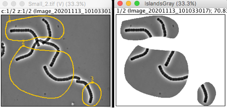
Fig 2: Define islands of interest: exclude problematic areas.
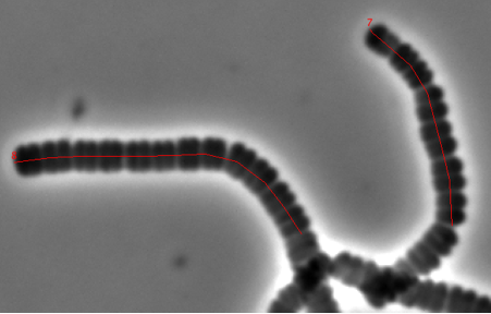
Fig 3: Mark Filament axes.
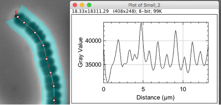
Fig 4: Finding maxima in Axis profile to resolve cells. Peak positions have sub-pixel resolution due to gauss-fitting.
.
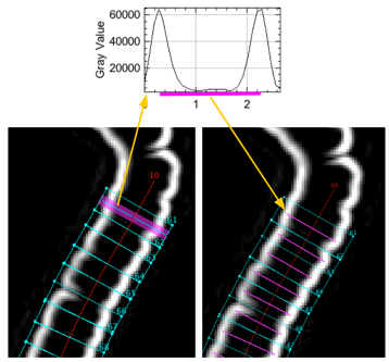
Fig 5: Finding maxima in Sobel-filtered image to detect cell length.
Peak positions have sub-pixel resolution due to gauss-fitting.
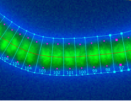
Fig 6: Resolved cell boxes as local coordinate systems.
The magenta dots are end points of the cell lengths, the connection line is here set to 'invisible'.
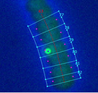
Fig 7: BSpots are marked with blue dot in channel 2.
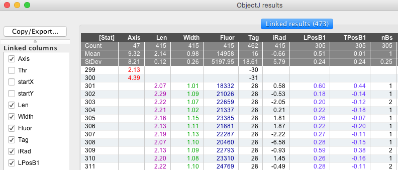
Fig 8: ObjectJ Results Table.
ObjectJ>Show ObjectJ Results:
| Column Ttitle | Meaning |
|---|---|
| Axis: | length of red filament axis |
| Thr: | threshold that was used by particle analyzer in chn 1 |
| StartX, StartY: | start point used by particle analyzer |
| Len: | cell length, distance between gradient maxima in channel 1 |
| Width: | width of the cell box at cell center (not at center of Len object) |
| Fluor: | mean intensity of the cell box in channel 2 |
| Tag: | cell-filament identifier (negative for filaments, positive for cells to identify the "owner"-filament) |
| iRad: | inverse bending radius (1000/rad, [ px-1 ]), if positive: numbered pole at convex side |
| LPosB1: | relative position (-0.1 .. 1.1) of strongest "BSpot" projected onto "Len" |
| TPosB1: | relative offset (-0.5 .. 0.5) from strongest "BSpot" to "Len" |
| nBs: | number of BSpots per cell |
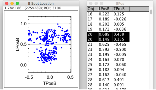
Fig 9: Output of ObjectJ>Calc B Positions.
Object #20 has 2 BSpots.